13. Analysis Algorithms¶

EPANET uses a variety of algorithms for the hydraulic and water quality analysis. This chapter describes the two different demand models used for hydraulics analysis and the algorithms for the water quality analysis.

13.1. Hydraulics¶

The method used in EPANET to solve the flow continuity and headloss equations that characterize the hydraulic state of the pipe network at a given point in time can be termed a hybrid node-loop approach. Todini and Pilati (1987) and later Salgado et al. (1988) chose to call it the “Gradient Method”. Similar approaches have been described by Hamam and Brameller (1971) (the “Hybrid Method) and by Osiadacz (1987) (the “Newton Loop-Node Method”). The only difference between these methods is the way in which link flows are updated after a new trial solution for nodal heads has been found. Because Todini’s approach is simpler, it was chosen for use in EPANET.

Todini (2003) describes how the Gradient Method can be extended to simulate pressure driven demands (PDD). The latest version of EPANET has been updated to include these capabilities. A water distribution pipe network can now be analyzed two ways, 1) assuming demand, and 2) assuming pressure driven demands. The subsections that follow provide a technical description for these two demand models.

Fixed Demand Model

Assume we have a pipe network with \({N}\) junction nodes and \({NF}\) fixed grade nodes (tanks and reservoirs). Let the flow-headloss relation in a pipe between nodes \(i\) and \(j\) be given as:

(13.1)¶\[H_{i} - H_{j} = h_{ij} = rQ_{ij}^{n} + mQ_{ij}^{2}\]

where \(H\) = nodal head, \(h\) = headloss, \(r\) = resistance coefficient, \(Q\) = flow rate, \(n\) = flow exponent, and \(m\) = minor loss coefficient. The value of the resistance coefficient will depend on which friction headloss formula is being used (see below). For pumps, the headloss (negative of the head gain) can be represented by a power law of the form

\[{h}_{ij} = {-\omega}^{2} ( {h}_{0} - r { ( {Q}_{ij}/{\omega} )}^{2 } )\]

where \(h_{0}\) is the shutoff head for the pump, \(\omega\) is a relative speed setting, and \(r\) and \(n\) are the pump curve coefficients. The second set of equations that must be satisfied is flow continuity around all nodes:

(13.2)¶\[\begin{split} \sum_{j} {Q}_{ij} - {D}_{i} = 0 \\ \mathit{for\ i = 1,... N}\end{split}\]

where \(D_{i}\) is the flow demand at node \(i\) and by convention, flow into a node is positive. For a set of known heads at the fixed grade nodes, we seek a solution for all heads \(H_{i}\) and flows \(Q_{ij}\) that satisfy Eqs. (13.1) and (13.2).

The Gradient solution method begins with an initial estimate of flows in each pipe that may not necessarily satisfy flow continuity. At each iteration of the method, new nodal heads are found by solving the matrix equation:

(13.3)¶\[\boldsymbol{AH} = \boldsymbol{F}\]

where \(A\) = an \((NxN)\) Jacobian matrix, \(H\) = an \((Nx1)\) vector of unknown nodal heads, and \(F\) = an \((Nx1)\) vector of right hand side terms.

The diagonal elements of the Jacobian matrix are:

\[{A}_{ij}= \sum_{j} \frac{1}{g_{ij}}\]

while the non-zero, off-diagonal terms are:

\[{A}_{ij} = -\frac{1}{g_{ij}}\]

where \(g_{ij}\) is the derivative of the headloss in the link between nodes \(i\) and \(j\) with respect to flow. For pipes, when resistance coefficient is not a function of flow rate,

\[{g}_{ij} = nr {{ | Q_{ij} | }^{n - 1}} + 2m | Q_{ij} |\]

when resistance coefficient is a function of flow rate, specifically as in Darcy-Weisbach head loss equation and when flow is turbulent,

\[{g}_{ij} = nr {{ | Q_{ij} | }^{n - 1}} + \frac{\partial r}{\partial Q_{ij}}|Q_{ij}|^n + 2m | Q_{ij} |\]

Zero flows can cause numerical instability in the GGA solver (Gorev et al., 2013; Elhay and Simpson, 2011). When flow approaches zero, a linear relationship is assumed between head loss and flow to prevent \({g}_{ij}\) from reaching zero. The value of \({g}_{ij}\) is capped at a specific value when the flow is smaller than what is defined by the specific \({g}\).

while for pumps

\[{g}_{ij} = n \omega^{2} r ({Q}_{ij}/{\omega} )^{n-1}\]

Each right hand side term consists of the net flow imbalance at a node plus a flow correction factor:

(13.4)¶\[{F}_{i} = \sum_{{j}} \left( Q_{ij} + \frac{y_{ij}}{g_{ij}} \right) - {D}_{i} + \sum_{f} \frac{H_{f}}{g_{ij}}\]

where the last term applies to any links connecting node \(i\) to a fixed grade node \(f\) and the flow correction factor \(y_{ij}\) is:

\[y_{ij} = ( r{ | {Q}_{ij} | }^{n} + m { | {Q}_{ij} | }^{2} )sgn ( {Q}_{ij} )\]

for pipes and

\[y_{ij} = - {\omega}^{2} ( {h}_{0} - r { ( { Q}_{ij }/{\omega} ) }^{n} )\]

for pumps, where \(sgn(x)\) is \(1\) if \(x > 0\) and \(-1\) otherwise (\(Q_{ij}\) is always positive for pumps).

After new heads are computed by solving Eq. (13.3), new flows are found from:

(13.5)¶\[{Q}_{ij} = {Q}_{ij} - \frac{1}{g_{ij}} ( y_{ij} - {H}_{i} - {H}_{j} )\]

The flow update formula always results in flow continuity around each node after the first iteration.

Iterations continue until some suitable convergence criterion based on residual errors associated with (13.1) and (13.2) is met. If convergence does not occur then Eqs. (13.3) and (13.5) are solved again.

EPANET uses several different hydraulic convergence criteria. Versions 2.0 and earlier based accuracy on the absolute flow changes relative to the total flow in all links. Gorev et al. (2013), however, observed that this criterion did not guarantee convergence towards the exact solution and proposed two new ones based on max head error and max flow change. These two criteria have been added to EPANET v2.2 as options that provide more rigorous control over hydraulic convergence.

Pressure Driven Demand Model

Now consider the case where the demand at a node \(i\), \(d_{i}\), depends on the pressure head \(p_{i}\) available at the node (where pressure head is hydraulic head \(h_{i}\) minus elevation \(E_{i}\)). There are several different forms of pressure dependency that have been proposed. Here we use Wagner’s equation (Wagner et al., 1988):

(13.6)¶\[\begin{split}d_{i} = \left\{ \begin{array}{l l} D_{i} & p_{i} \ge P_{f} \\ D_{i} \left( \frac{p_{i} - P_{0}}{P_{f} - P_{0}} \right) ^{e} & P_{0} < p_i < P_{f} \\ 0 & p_{i} \le P_{0} \end{array} \right.\end{split}\]

\(D_{i}\) is the full normal demand at node \(i\) when the pressure \(p_{i}\) equals or exceeds \(P_{f}\), \(P_{0}\) is the pressure below which the demand is 0, and \(e\) is an exponent usually set equal to 0.5 (to mimic flow through an orifice).

Eq. (13.6) can be inverted to express head loss through a virtual link as a function of the demand flowing out of node \(i\) to a virtual reservoir with fixed pressure head \(P_{0} + E_{i}\):

(13.7)¶\[ h_{i} - P_{0} - E_{i} = R_{di} d_{i}^{e}\]

where \(E_{i}\) is the node’s elevation and \(R_{di} = (P_{f} - P_{0})/D_{i}^{e}\) is the link’s resistance coefficient. This expression can be folded into the GGA matrix equations, where the pressure driven demands \(d_{i}\) are treated as the unknown flows in the virtual links that honor constraints in Eq. (13.6).

The head loss \(h_{d}\) and its gradient \(g_{d}\) through the virtual link can be evaluated as follows (with node subscripts suppressed for clarity):

If the current demand flow \(d\) is greater than the full Demand \(D\):

\[\begin{split}\begin{gathered} h_{d} = R_{d} D^{e} + R_{\text{HIGH}}(d - D) \\ g_{d} = R_{\text{HIGH}} \end{gathered}\end{split}\]

where \(R_{\text{HIGH}}\) is a large resistance factor (e.g. 10⁹).

Otherwise Eq. (13.7) is used to evaluate the head loss and gradient:

\[\begin{split}\begin{gathered} g_{d} = e R_{d} \left| d \right|^{e - 1} \\ h_{d} = g_{d} d / e \end{gathered}\end{split}\]

and a one-sided barrier function \(h_{b}(d)\) and its derivative \(g_{b}(d)\) is added onto \(h_{d}\) and \(g_{d}\), respectively, to prevent \(d\) from going negative.

The aforementioned barrier function has the form:

\[\begin{split}\begin{gathered} h_{b} = \ \left( a - \sqrt{a^{2} + \epsilon^{2}} \right)/2 \\ g_{b} = \left( R_{\text{HIGH}}/2 \right)\left( 1 - a/\sqrt{a^{2} + \epsilon^{2}} \right) \end{gathered}\end{split}\]

where \(a = R_{\text{HIGH}}d\) and \(\epsilon\) is a small tolerance (e.g., 10^-3).

These head loss and gradient values are then incorporated into the normal set of GGA matrix equations as follows:

For the diagonal entry of \(A\) corresponding to node i:

\[A_{ii} = A_{ii} + 1/g_{di}\]

For the entry of \(F\) corresponding to node \(i\):

\[F_{i} = F_{i} + D_{i} - d_{i} + \left( h_{di} + E_{i} + P_{0} \right) / g_{di}\]

Note that \(D_{i}\) is added to \(F_{i}\) to cancel out having subtracted it from the original \(F_{i}\) value appearing in Eq. (13.4).

After a new set of nodal heads is found, the demands at node \(i\) are updated using Eq. (13.5) which takes the form:

\[d_{i} = d_{i} - ( h_{di} - h_{i} + E_{i} + P_{0} ) / g_{di}\]

The following assumptions apply to the implementation of PDD in EPANET:

A global set of minimum \(P_{0}\) and full \(P_{f}\) (or nominal) pressure limits apply to all nodes.

In extended period analysis, where the full demands change at different time periods, the same pressure driven demand function is applied to the current full demand (instead of changing \(P_{f}\) to accommodate changes in \(D_{f}\) ).

EPANET Implementation

EPANET implements the fixed demand and PDD models for hydraulics using the procedure outlined in this section.
The linear system of equations (13.3) is solved using a sparse matrix method based on multiple minimum-degree node re-ordering (Liu 1985). After re-ordering the nodes to minimize the amount of fill- in for matrix \(A\), a symbolic factorization is carried out so that only the non-zero elements of A need be stored and operated on in memory. For extended period simulation this re-ordering and factorization is only carried out once at the start of the analysis.

For the very first iteration, the flow in a pipe is chosen equal to the flow corresponding to a velocity of 1 ft/sec, while the flow through a pump equals the design flow specified for the pump. (All computations are made with head in feet and flow in cfs).

The resistance coefficient for a pipe (\(r\)) is computed as described in Table 3.1. For the Darcy-Weisbach headloss equation, the friction factor \(f\) is computed by different equations depending on the flow’s Reynolds Number (\(Re\)):

Hagen – Poiseuille formula for \(Re < 2,000\) (Bhave, 1991):

\[f = \frac{64}{Re}\]

Swamee and Jain approximation to the Colebrook - White equation for Re > 4,000 (Bhave, 1991):

\[f = \frac{0.25}{{ \left[ \ln \left( \frac{\epsilon}{3.7d} + \frac{5.74}{{Re}^{0.9} } \right) \right] }^{2}}\]

Cubic Interpolation From Moody Diagram for \(2,000 < Re < 4,000\) (Dunlop, 1991):

\[\begin{split}\begin{gathered} f = (X1 + R (X2 + R (X3 + X4))) \\ R = \frac{Re}{2000} \end{gathered}\end{split}\]

\[\begin{split}\begin{gathered} X1 = 7FA - FB \\ X2 = 0.128 - 17 FA + 2.5 FB \\ X3 = -0.128 + 13 FA - 2 FB \\ X4 = R ( 0.032 - 3 FA + 0.5 FB ) \\ FA = { ( Y3 )}^{-2} \\ FB = FA ( 2 - \frac{0.00514215} {( Y2 ) ( Y3 ) } ) \\ Y2 = \frac{\epsilon} {3.7d} + \frac{5.74}{{Re}^{0.9}} \\ Y3 = -0.86859 \ln \left( \frac{\epsilon}{3.7d} + \frac{5.74}{{4000}^{0.9}} \right) \end{gathered}\end{split}\]

where \(\epsilon\) = pipe roughness and \(d\) = pipe diameter.

Based on friction factor equations described above and Darcy-Weisbach equation in Table 3.1, resistance coefficient is not a function of flow and linear relationship exists between head loss and flow when Re > 2000. If Re > 2000, resistance coefficient depends on pipe flow and the sensitivity of resistance coefficient to flow needs to be computed in order to calculate \({g}_{ij}\) for the pipe.

The minor loss coefficient based on velocity head (\(K\)) is converted to one based on flow (\(m\)) with the following relation:

\[m = \frac{ 0.02517K} {d^{4}}\]

Emitters at junctions are modeled as a fictitious pipe between the junction and a fictitious reservoir. The pipe’s headloss parameters are \(n = (1/\gamma)\), \(r = (1/C)^n\), and \(m = 0\) where \(C\) is the emitter’s discharge coefficient and \(\gamma\) is its pressure exponent. The head at the fictitious reservoir is the elevation of the junction. The computed flow through the fictitious pipe becomes the flow associated with the emitter.

Open valves are assigned an \(r\)- value by assuming the open valve acts as a smooth pipe (\(f = 0.02\)) whose length is twice the valve diameter. Closed links are assumed to obey a linear headloss relation with a large resistance factor, i.e., \(h = 10^{8} Q\), so that \(p = 10^{-8}\) and \(y = Q\). For links where \((r + m)Q < 10^{-7}\), \(p = 10^{7}\) and \(y = Q/n\).

Status checks on pumps, check valves (CVs), flow control valves, and pipes connected to full/empty tanks are made after every other iteration, up until the 10th iteration. After this, status checks are made only after convergence is achieved. Status checks on pressure control valves (PRVs and PSVs) are made after each iteration.

During status checks, pumps are closed if the head gain is greater than the shutoff head (to prevent reverse flow). Similarly, check valves are closed if the headloss through them is negative (see below). When these conditions are not present, the link is re-opened. A similar status check is made for links connected to empty/full tanks. Such links are closed if the difference in head across the link would cause an empty tank to drain or a full tank to fill. They are re- opened at the next status check if such conditions no longer hold.
Simply checking if \(h < 0\) to determine if a check valve should be closed or open was found to cause cycling between these two states in some networks due to limits on numerical precision. The following procedure was devised to provide a more robust test of the status of a check valve (CV):
if |h| > Htol then
  if h < -Htol then     status = CLOSED
  if Q < -Qtol then     status = CLOSED
  else                  status = OPEN

else
  if *Q* < -Qtol then   status = CLOSED
  else                  status = unchanged
where Htol = 0.0005 ft and Qtol = 0.001 cfs.
If the status check closes an open pump, pipe, or CV, its flow is set to \(10^{-6}\) cfs. If a pump is re-opened, its flow is computed by applying the current head gain to its characteristic curve. If a pipe or CV is re- opened, its flow is determined by solving Eq. (13.1) for \(Q\) under the current headloss \(h\), ignoring any minor losses.

Matrix coefficients for pressure breaker valves (PBVs) are set to the following: \(p = 10^{8}\) and \(y = 10^{8} Hset\), where \(Hset\) is the pressure drop setting for the valve (in feet). Throttle control valves (TCVs) are treated as pipes with \(r\) as described in item 6 above and \(m\) taken as the converted value of the valve setting (see item 4 above).

Matrix coefficients for pressure reducing, pressure sustaining, and flow control valves (PRVs, PSVs, and FCVs) are computed after all other links have been analyzed. Status checks on PRVs and PSVs are made as described in item 7 above. These valves can either be completely open, completely closed, or active at their pressure or flow setting.
The logic used to test the status of a PRV is as follows:
If current status = ACTIVE then
  if Q < -Qtol then              new status = CLOSED
  if Hi < Hset + Hml – Htol then new status = OPEN
                            else new status = ACTIVE

If curent status = OPEN then
  if Q < -Qtol then              new status = CLOSED
  if Hi > Hset + Hml + Htol then new status = ACTIVE
                            else new status = OPEN

If current status = CLOSED then
  if  Hi > Hj + Htol
  and Hi < Hset – Htol      then new status = OPEN

  if  Hi > Hj + Htol
  and Hj < Hset - Htol      then new status = ACTIVE
                            else new status = CLOSED
where Q is the current flow through the valve, Hi is its upstream head, Hj is its downstream head, Hset is its pressure setting converted to head, Hml is the minor loss when the valve is open (= mQ²), and Htol and Qtol are the same values used for check valves in item 9 above. A similar set of tests is used for PSVs, except that when testing against Hset, the i and j subscripts are switched as are the > and < operators.
Flow through an active PRV is maintained to force continuity at its downstream node while flow through a PSV does the same at its upstream node. For an active PRV from node i to j:

\[\frac{1}{g_{ij}} = 0\]

\[{F}_{j} = {F}_{j} + {10}^{8} Hset\]

\[{A}_{jj} = {A}_{jj} + {10}^{8}\]

This forces the head at the downstream node to be at the valve setting Hset. An equivalent assignment of coefficients is made for an active PSV except the subscript for F and A is the upstream node i. Coefficients for open/closed PRVs and PSVs are handled in the same way as for pipes.

For an active FCV from node i to j with flow setting Qset, Qset is added to the flow leaving node i and entering node j, and is subtracted from Fi and added to Fj. If the head at node i is less than that at node j, then the valve cannot deliver the flow and it is treated as an open pipe.

After initial convergence is achieved (flow convergence plus no change in status for PRVs and PSVs), another status check on pumps, CVs, FCVs, and links to tanks is made. Also, the status of links controlled by pressure switches (e.g., a pump controlled by the pressure at a junction node) is checked. If any status change occurs, the iterations must continue for at least two more iterations (i.e., a convergence check is skipped on the very next iteration). Otherwise, a final solution has been obtained.

For extended period simulation (EPS), the following procedure is implemented:

After a solution is found for the current time period, the time step for the next solution is the minimum of:

The time until a new demand period begins

The shortest time for a tank to fill or drain,

The shortest time until a tank level reaches a point that triggers a change in status for some link (e.g., opens or closes a pump) as stipulated in a simple control

The next time until a simple timer control on a link kicks in

The next time at which a rule-based control causes a status change somewhere in the network

In computing the times based on tank levels, the latter are assumed to change in a linear fashion based on the current flow solution. The activation time of rule-based controls is computed as follows:

Starting at the current time, rules are evaluated at a rule time step. Its default value is 1/10 of the normal hydraulic time step (e.g., if hydraulics are updated every hour, then rules are evaluated every 6 minutes).

Over this rule time step, clock time is updated, as are the water levels in storage tanks (based on the last set of pipe flows computed).

If a rule’s conditions are satisfied, then its actions are added to a list. If an action conflicts with one for the same link already on the list then the action from the rule with the higher priority stays on the list and the other is removed. If the priorities are the same then the original action stays on the list.

After all rules are evaluated, if the list is not empty then the new actions are taken. If this causes the status of one or more links to change then a new hydraulic solution is computed and the process begins anew.

If no status changes were called for, the action list is cleared and the next rule time step is taken unless the normal hydraulic time step has elapsed.

Time is advanced by the computed time step, new demands are found, tank levels are adjusted based on the current flow solution, and link control rules are checked to determine which links change status.

A new set of iterations with Eqs. (13.3) and (13.5) are begun at the current set of flows.

13.2. Water Quality¶

The governing equations for EPANET’s water quality solver are based on the principles of conservation of mass coupled with reaction kinetics. The following phenomena are represented (Rossman et al., 1993; Rossman and Boulos, 1996):

Advective Transport in Pipes

A dissolved substance will travel down the length of a pipe with the same average velocity as the carrier fluid while at the same time reacting (either growing or decaying) at some given rate. Longitudinal dispersion is usually not an important transport mechanism under most operating conditions. This means there is no intermixing of mass between adjacent parcels of water traveling down a pipe. Advective transport within a pipe is represented with the following equation:

(13.8)¶\[\frac{ \partial {C}_{i}} {\partial t} = - u_{i} \frac{\partial{C}_{i}}{\partial x} + r({C}_{i})\]

where \(C_i\) = concentration (mass/volume) in pipe \(i\) as a function of distance \(x\) and time \(t\), \(u_i\) = flow velocity (length/time) in pipe \(i\), and \(r\) = rate of reaction (mass/volume/time) as a function of concentration.

Mixing at Pipe Junctions

At junctions receiving inflow from two or more pipes, the mixing of fluid is taken to be complete and instantaneous. Thus the concentration of a substance in water leaving the junction is simply the flow-weighted sum of the concentrations from the inflowing pipes. For a specific node \(k\) one can write:

(13.9)¶\[C_{i|x=0} = \frac{\sum_{ j \in I_k} Q_{j} C_{j|x= L_j}+Q_{k,ext} C_{k,ext}} {\sum_{j \in I_k} Q_j + Q_{k,ext}}\]

where \(i\) = link with flow leaving node \(k\), \(I_k\) = set of links with flow into \(k\), \(L_j\) = length of link \(j\), \(Q_j\) = flow (volume/time) in link \(j\), \(Q_k,ext\) = external source flow entering the network at node \(k\), and \(C_k,ext\) = concentration of the external flow entering at node \(k\). The notation \(C_i|x=0\) represents the concentration at the start of link \(i\), while \(C_i|x=L\) is the concentration at the end of the link.

Mixing in Storage Facilities

It is convenient to assume that the contents of storage facilities (tanks and reservoirs) are completely mixed. This is a reasonable assumption for many tanks operating under fill-and-draw conditions providing that sufficient momentum flux is imparted to the inflow (Rossman and Grayman, 1999). Under completely mixed conditions the concentration throughout the tank is a blend of the current contents and that of any entering water. At the same time, the internal concentration could be changing due to reactions. The following equation expresses these phenomena:

(13.10)¶\[\frac{\partial ({V}_{s} {C}_{s}) }{\partial t} = \sum_{i \in I_{s}} {Q}_{i}{C}_{i | x={L}_{i}} - \sum_{j \in O_{s}} {Q}_{j}{C}_{s} + r({C}_{s})\]

where \(V_s\) = volume in storage at time \(t\), \(C_s\) = concentration within the storage facility, \(I_s\) = set of links providing flow into the facility, and \(O_s\) = set of links withdrawing flow from the facility.

Bulk Flow Reactions

While a substance moves down a pipe or resides in storage it can undergo reaction with constituents in the water column. The rate of reaction can generally be described as a power function of concentration:

\[r = k{ C}^{n }\]

where \(k\) = a reaction constant and \(n\) = the reaction order. When a limiting concentration exists on the ultimate growth or loss of a substance then the rate expression becomes

\[\begin{split}\begin{gathered} R = {K}_{b} ({C}_{L}-C) {C}^{n-1} \\ \mathit{for\ n > 0, K_b > 0} \end{gathered}\end{split}\]

\[\begin{split}\begin{gathered} R = {K}_{b} (C - {C}_{L} ) {C}^{n - 1} \\ \mathit{for\ n > 0, K_b < 0} \end{gathered}\end{split}\]

where \(C_L\) = the limiting concentration.

Some examples of different reaction rate expressions are:

Simple First-Order Decay (\(C_L = 0, K_b < 0, n = 1\)):

\[R = {K}^{b}C\]

The decay of many substances, such as chlorine, can be modeled adequately as a simple first-order reaction.

First-Order Saturation Growth (\(C_L > 0, K_b > 0, n = 1\)):

\[R = {K}_{b} ( {C}_{L} - C )\]

This model can be applied to the growth of disinfection by-products, such as trihalomethanes, where the ultimate formation of by-product (\(C_L\)) is limited by the amount of reactive precursor present.

Two-Component, Second Order Decay (\(C_L \neq 0, K_b < 0, n = 2\)):

\[R = {K}_{b} C({C}_{L} - C)\]

This model assumes that substance A reacts with substance B in some unknown ratio to produce a product P. The rate of disappearance of A is proportional to the product of A and B remaining. \(C_L\) can be either positive or negative, depending on whether either component A or B is in excess, respectively. Clark (1998) has had success in applying this model to chlorine decay data that did not conform to the simple first-order model.

Michaelis-Menton Decay Kinetics (\(C_L > 0, K_b < 0, n < 0\)):

\[R = \frac{{K}_{b}C} {{C}_{L} - C}\]

As a special case, when a negative reaction order n is specified, EPANET will utilize the Michaelis-Menton rate equation, shown above for a decay reaction. (For growth reactions the denominator becomes \(C_L + C\).) This rate equation is often used to describe enzyme-catalyzed reactions and microbial growth. It produces first- order behavior at low concentrations and zero-order behavior at higher concentrations. Note that for decay reactions, \(C_L\) must be set higher than the initial concentration present.

Koechling (1998) has applied Michaelis-Menton kinetics to model chlorine decay in a number of different waters and found that both \(K_b\) and \(C_L\) could be related to the water’s organic content and its ultraviolet absorbance as follows:

\[{K}_{b} = -0.32\ UVA^{1.365 }\frac{( 100\ UVA )} {DOC}\]

\[{C}_{L} = 4.98\ UVA - 1.91\ DOC\]

where \(UVA\) = ultraviolet absorbance at 254 nm (1/cm) and \(DOC\) = dissolved organic carbon concentration (mg/L).

Note: These expressions apply only for values of \(K_b\) and \(C_L\) used with Michaelis-Menton kinetics.

Zero-Order growth (\(C_L = 0, K_b = 1, n = 0\))

\[R = 1.0\]

This special case can be used to model water age, where with each unit of time the “concentration” (i.e., age) increases by one unit.

The relationship between the bulk rate constant seen at one temperature (T1) to that at another temperature (T2) is often expressed using a van’t Hoff - Arrehnius equation of the form:

\[{K}_{b2}={K}_{b1}{\theta}^{T2 - T1}\]

where \(\theta\) is a constant. In one investigation for chlorine, \(\theta\) was estimated to be 1.1 when \(T1\) was 20 deg. C (Koechling, 1998).

Pipe Wall Reactions

While flowing through pipes, dissolved substances can be transported to the pipe wall and react with material such as corrosion products or biofilm that are on or close to the wall. The amount of wall area available for reaction and the rate of mass transfer between the bulk fluid and the wall will also influence the overall rate of this reaction. The surface area per unit volume, which for a pipe equals 2 divided by the radius, determines the former factor. The latter factor can be represented by a mass transfer coefficient whose value depends on the molecular diffusivity of the reactive species and on the Reynolds number of the flow (Rossman et. al, 1994). For first- order kinetics, the rate of a pipe wall reaction can be expressed as:

\[r = \frac{ 2 k_w k_f C } { R (k_w + k_f) }\]

where \(k_w\) = wall reaction rate constant (length/time), \(k_f\) = mass transfer coefficient (length/time), and \(R\) = pipe radius. For zero-order kinetics the reaction rate cannot be any higher than the rate of mass transfer, so

\[r = \min ( k_w, k_f C) ( 2/R )\]

where \(k_w\) now has units of mass/area/time.

Mass transfer coefficients are usually expressed in terms of a dimensionless Sherwood number (\(Sh\)):

\[{k}_{f} = Sh \frac{D}{d}\]

in which \(D\) = the molecular diffusivity of the species being transported (length ² /time) and \(d\) = pipe diameter. In fully developed laminar flow, the average Sherwood number along the length of a pipe can be expressed as

\[Sh = 3.65 + \frac{0.0668 ( d/L )Re\ Sc} {1 + 0.04{ [ ( d/L )Re\ Sc ]}^{2/3}}\]

in which \(Re\) = Reynolds number and \(Sc\) = Schmidt number (kinematic viscosity of water divided by the diffusivity of the chemical) (Edwards et.al, 1976). For turbulent flow the empirical correlation of Notter and Sleicher (1971) can be used:

\[Sh = 0.0149{Re}^{0.88}{Sc}^{1/3}\]

System of Equations

When applied to a network as a whole, Eqs. (13.8) - (13.10) represent a coupled set of differential/algebraic equations with time-varying coefficients that must be solved for \(C_i\) in each pipe \(i\) and \(C_s\) in each storage facility \(s\). This solution is subject to the following set of externally imposed conditions:

Initial conditions that specify \(C_i\) for all \(x\) in each pipe \(i\) and \(C_s\) in each storage facility \(s\) at time 0

Boundary conditions that specify values for \(C_k,ext\) and \(Q_k,ext\) for all time \(t\) at each node \(k\) which has external mass inputs

Hydraulic conditions which specify the volume \(V_s\) in each storage facility \(s\) and the flow \(Q_i\) in each link \(i\) at all times \(t\)

Lagrangian Transport Algorithm

EPANET’s water quality simulator uses a Lagrangian time-based approach to track the fate of discrete parcels of water as they move along pipes and mix together at junctions between fixed-length time steps (Liou and Kroon, 1987). These water quality time steps are typically much shorter than the hydraulic time step (e.g., minutes rather than hours) to accommodate the short times of travel that can occur within pipes. As time progresses, the size of the most upstream segment in a pipe may increase as water enters the pipe while an equal loss in size of the most downstream segment occurs as water leaves the link; therefore, the total volume of all the segments within a pipe does not change and the size of the segments between these leading and trailing segments remains unchanged (see Fig. 13.1).

The following steps occur within each such time step:

The water quality in each segment is updated to reflect any reaction that may have occurred over the time step.

For each node in topological order (from upstream to downstream):

If the node is a junction or tank, the water from the leading segments of the links with flow into it, if not zero, is blended together to compute a new water quality value. The volume contributed from each segment equals the product of its link’s flow rate and the time step. If this volume exceeds that of the segment, then the segment is destroyed and the next one in line behind it begins to contribute its volume.

If the node is a junction its new quality is computed as its total mass inflow divided by its total inflow volume. If it is a tank, its quality is updated depending on the method used to model mixing in the tank (see below).

The node’s concentration is adjusted by any contributions made by external water quality sources.

A new segment is created in each link with flow out of the node. Its volume equals the product of the link flow and the time step and its quality equals the new quality value computed for the node.

To cut down on the number of segments, new ones are only created if the new node quality differs by a user-specified tolerance from that of the last segment in the outflow link. If the difference in quality is below the tolerance, then the size of the current last segment in the link is simply increased by the volume flowing into the link over the time step and the segment quality is a volume-weighted average of the node and segment quality.

This process is then repeated for the next water-quality time step. At the start of the next hydraulic time step any link experiencing a flow reversal has the order of its segments reversed and if any flow reversal occurs the network’s nodes are re-sorted topologically, from upstream to downstream. Sorting the nodes topologically allows the method to conserve mass and reduce the potential mass balance error experienced with EPANET 2.0 (Davis et al., 2018) even when very short pipes or zero-length pumps and valves are encountered. Initially each pipe in the network consists of a single segment whose quality equals the initial quality assigned to the upstream node.

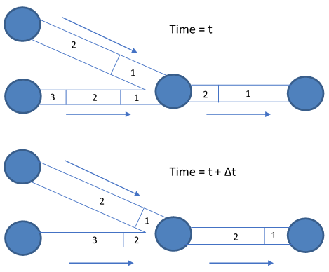
Fig. 13.1 Behavior of segments in the Lagrangian solution method.